How to Use VLOOKUP in Numbers: A Step-by-Step Guide for Numbers Users

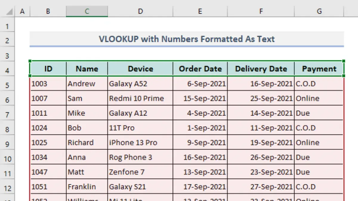
Imagine you're managing a budget in Apple Numbers and need to quickly find specific values from a large table. Instead of manually scanning through rows, you want a reliable way to pull data by matching certain criteria. This is where understanding how to use VLOOKUP in Numbers becomes invaluable.

This article guides you step-by-step through using VLOOKUP within Apple Numbers, focusing on searching for numbers, text, or a combination of both. You'll learn how to set up your formulas correctly, use the $ symbol to fix ranges, count data using VLOOKUP, and troubleshoot common issues unique to Numbers versus Excel.

Key takeaways

• VLOOKUP in Numbers requires careful range selection and exact matches for accurate results.
• Combining numbers and text in lookup values needs consistent formatting to avoid errors.
• Using the $ symbol locks ranges, preventing errors when copying formulas.
• You can count occurrences by combining VLOOKUP with other functions in Numbers.
• Troubleshooting often involves checking data types and ensuring no extra spaces or hidden characters.

Before you start: What you need to use VLOOKUP in Numbers

To use VLOOKUP effectively in Apple Numbers, first make sure you have the app installed on your Mac, iPad, or iPhone. This function works within your spreadsheet to search for a value in one column and return a corresponding value from another column. Prepare a dataset that includes at least two columns: one for the lookup values and another for the results you want to retrieve. For example, a simple table might list product IDs in the first column and product names in the second.

Understanding the VLOOKUP function structure is essential. The syntax in Numbers is =VLOOKUP(search-for, lookup-table, result-column, approximate). Here, search-for is the value you want to find, lookup-table is the range including both lookup and result columns, result-column is the number of the column in that range containing the value to return, and approximate is a TRUE or FALSE value indicating whether to find an approximate match or an exact match.

You should know the difference between exact and approximate matches: use FALSE for exact matches to find the precise value, and TRUE for approximate matches when working with sorted numerical data. Choosing the right mode prevents errors or incorrect results.

1. Open Apple Numbers and load your spreadsheet with data organized into columns. You should see your dataset clearly, for example, product IDs in column A and product names in column B.
2. Select the cell where you want the VLOOKUP result to appear.
3. Enter a basic VLOOKUP formula like =VLOOKUP("12345", A:B, 2, FALSE). This searches for "12345" in the first column of A:B and returns the corresponding product name from the second column.
4. Press Return. If the lookup value exists, the result cell will display the matching data from the second column.

This setup ensures you are ready to apply VLOOKUP confidently in Numbers without confusion from Excel-specific differences.

How to do a basic VLOOKUP with numbers in Apple Numbers

To perform a straightforward VLOOKUP using numerical values in Apple Numbers, you start by selecting the cell where you want the result to appear. This will be the cell that displays the information retrieved from your lookup table. Next, you enter the VLOOKUP formula, specifying your numerical lookup value directly in the formula.

For example, imagine you have a table listing product IDs in the first column and product names in the second. If you want to find the name of the product with ID 102, you will use 102 as your lookup value. You then define the table range that contains both product IDs and names, and specify which column index to return. Since the product names are in the second column, you use 2 as the column index.

It is important to set the match type to exact match to avoid incorrect or approximate results. This ensures Numbers looks for exactly the number you specify, not a close or nearest value, which may cause confusion.

1. Select the cell where you want the product name to appear. After this, the cell will be ready to receive the formula.
2. Enter the formula: =VLOOKUP(102, A2:B10, 2, FALSE). Here, 102 is the number you are searching for, A2:B10 is the range containing your product IDs and names, 2 is the column index for product names, and FALSE indicates an exact match is required.
3. Press Return. The cell should now display the product name associated with ID 102, for example, "Wireless Mouse".
4. If the formula returns an error or unexpected result, double-check the range and ensure the lookup value is present exactly in the first column of the table range.

How to use VLOOKUP with text and numbers combined

Apple Numbers treats text and numbers differently when performing lookups, which can cause confusion if your lookup values or table data mix both types. For example, the number 123 and the text "123" are not automatically considered the same. This distinction can lead to VLOOKUP returning errors or incorrect results when you try to match alphanumeric codes or IDs.

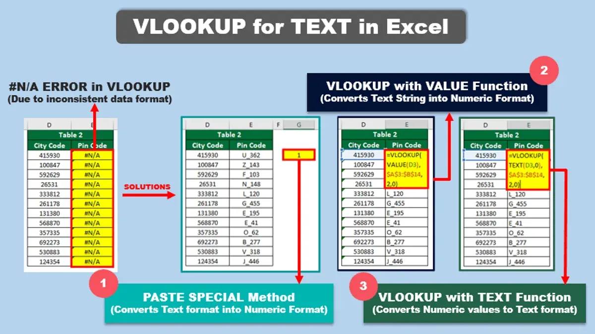
To handle this, you can normalize your lookup values and table data by converting numbers to text or combining text and numbers consistently. Using the TEXT() function or concatenation helps ensure that both the lookup value and the table’s corresponding column have matching formats.

1. Identify the column containing mixed text and numbers in your lookup table. For example, a product ID like "A123" or a code like "X45".
2. In a helper column next to your table, create a formula to convert those values to text uniformly, such as =TEXT(A2, "@") or concatenate with an empty string: =A2 & "". You should see the original data converted explicitly to text.
3. Use the same text conversion on your lookup value in the VLOOKUP formula. For example, instead of =VLOOKUP(B2, Table 1::A:C, 2, FALSE), write =VLOOKUP(TEXT(B2, "@"), Table 1::D:F, 2, FALSE) where column D is the helper column with text-converted IDs.
4. After entering the formula, verify that VLOOKUP returns the correct matching value. Without text conversion, the formula often returns #N/A or incorrect results when mixing text and numbers.

By ensuring both lookup values and table data are text-formatted consistently, you avoid mismatches caused by Numbers’ strict type comparison. This approach works well for alphanumeric IDs, codes, or any data mixing letters and numbers.

How to use the $ symbol in VLOOKUP formulas to fix ranges

When you write a VLOOKUP formula in Apple Numbers, references to cells or ranges can be relative or absolute. Relative references adjust automatically when you copy the formula to another cell, while absolute references remain fixed. Understanding this difference is crucial to prevent errors, especially when your lookup table is a fixed range.

In VLOOKUP, the table range must stay constant as you copy the formula down or across your sheet. Without locking this range using the $ symbol, the reference shifts, causing the formula to look in the wrong place and return incorrect or missing results.

1. Click the cell with your VLOOKUP formula.
2. In the formula bar, locate the table range reference, for example, A2:B10.
3. Add $ before the column letters and row numbers to make the range absolute, like $A$2:$B$10.
4. Press Enter and then copy the formula to other cells.
5. Observe that the lookup range stays fixed, and the formula returns correct results for each lookup value.

For example, a formula without $ might look like this: =VLOOKUP(D2, A2:B10, 2, FALSE). When copied down, the range shifts to A3:B11, A4:B12, and so on, which often leads to errors.

In contrast, a formula with absolute references is written as =VLOOKUP(D2, $A$2:$B$10, 2, FALSE). Copying this keeps the range locked, ensuring consistent and accurate lookups.

How to perform VLOOKUP to count data in Numbers

VLOOKUP by itself does not count how many times a value appears in your data. However, you can combine it with counting functions like COUNTIF or SUMIF to summarize data based on lookup results. This approach is useful when you want to count orders, occurrences, or matches related to a lookup value found via VLOOKUP.

For example, suppose you have a list of orders with order IDs and product names, and you want to count how many orders correspond to a specific product found using VLOOKUP. You can set this up by using VLOOKUP to find the product name, then COUNTIF to count all orders matching that product.

1. Identify the lookup value you want to count occurrences for, such as a specific order ID or product code. For example, enter "A102" in cell D2. When done, you will see the lookup value in that cell.
2. Use VLOOKUP to retrieve the related product name from your main data table. Enter this formula in E2: =VLOOKUP(D2, Table1::A:B, 2, FALSE). When it works, the product name matching order ID A102 appears in E2.
3. In another cell, use COUNTIF to count how many times the product name from E2 appears in the product column of your data. For example, in F2, enter =COUNTIF(Table1::B, E2). This counts all orders for that product. You should see a number representing the total orders matching that product.
4. Optionally, you can combine these steps into one formula without a helper cell: =COUNTIF(Table1::B, VLOOKUP(D2, Table1::A:B, 2, FALSE)). This formula counts occurrences directly using VLOOKUP’s result.

By using VLOOKUP to find the lookup value and COUNTIF to tally occurrences, you can effectively summarize your data in Numbers. This method works similarly with SUMIF if you want to sum values related to your lookup instead of counting.

How to do VLOOKUP on a range of numbers in Apple Numbers

Using VLOOKUP to find values within a range of numbers in Apple Numbers requires activating approximate match mode. This mode allows you to look up a value that falls within a defined range rather than needing an exact match. To set this up, your lookup table should list the lower bounds of each range sorted in ascending order, with the corresponding results beside them.

For example, if you want to assign tax rates based on income brackets, create a table where the first column contains the minimum income for each bracket (such as 0, 10,000, 40,000), and the second column shows the tax rate for that bracket. When you use VLOOKUP with approximate match enabled, it will find the correct bracket for any income value.

1. Prepare your lookup table with range lower bounds in the first column sorted from smallest to largest. For example, list income thresholds like 0, 10,000, 40,000, and corresponding tax rates in the next column.
   When done correctly, the table clearly shows each range’s start value and result.
2. Enter the VLOOKUP formula using your lookup value (such as an income cell), the table range, the column index of the results, and set the last argument to TRUE for approximate match.
   If set correctly, Numbers will return the tax rate for the bracket your income falls into.
3. Test with several lookup values that fall into different ranges to confirm the formula returns expected results.
   Seeing different tax rates for different incomes confirms the approximate match works.

Keep in mind VLOOKUP’s approximate match only works if your lookup values and table are sorted correctly and you want the nearest lower range. It cannot handle overlapping or complex ranges directly. If you need more precise range checks or overlapping intervals, combining IF functions or using helper columns with Boolean logic may be necessary.

How to troubleshoot VLOOKUP not finding numbers or returning errors in Numbers

When VLOOKUP doesn't find your numbers or returns errors like #N/A or #REF!, the issue often lies in data types or formula setup. Start by ensuring your lookup value and the data in the first column of your lookup range are consistent in type—both should be numbers or both text. If one is formatted as text while the other is numeric, VLOOKUP will fail to find a match.

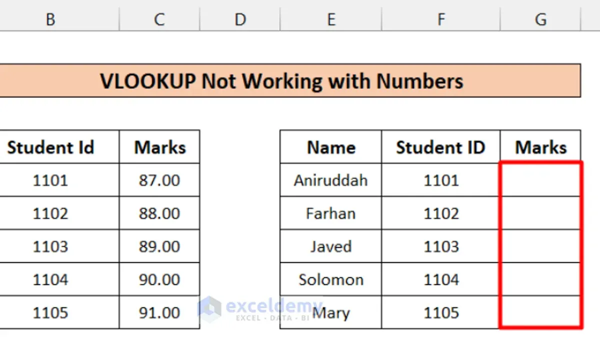
Next, verify that your lookup column is sorted if you are using approximate match mode (fourth parameter set to TRUE or omitted). An unsorted column here can cause incorrect or unexpected results. For exact matches, sorting is not required but data type consistency remains crucial.

Common errors include:

• #N/A: No exact match found. Check that the lookup value exists and matches the data type in the lookup column.
• #REF!: The column index number in the formula exceeds the number of columns in the lookup range. Adjust the column index to a valid number.
• Unexpected results: Caused by approximate match with unsorted data or mixing text and number formats.

To fix numbers formatted as text, select the cells, then use the Format panel to set the cell format explicitly to Number. Alternatively, use the VALUE() function on your lookup value or table data to convert text to numbers before using VLOOKUP.

1. Check the data type of your lookup value and the first column of your lookup table. They should both be numbers or both text. If they differ, reformat them to match.
   Success looks like VLOOKUP returning expected matching data instead of errors.
2. If using approximate match, ensure the lookup column is sorted in ascending order.
   Success means VLOOKUP returns a close match or correct range value.
3. Verify that the column index number in your formula is within the bounds of the specified table range.
   Success means no #REF! errors appear.
4. If you see #N/A, confirm the lookup value exists exactly in the lookup column and matches the data type.
   Success is finding the correct corresponding value.
5. Convert number-formatted-as-text cells by selecting them, opening the Format panel, and changing the format to Number.
   Success is VLOOKUP correctly recognizing these as numeric values.

Frequently asked questions

How to vlookup numbers in excel?

In Excel, you use the VLOOKUP function by specifying the lookup value, the table array, the column index number, and the range lookup type. For numbers, ensure the lookup value and the column data are formatted consistently as numbers to avoid mismatches. Also, use FALSE for an exact match when searching for specific numbers.

How to use $ in vlookup?

The $ symbol in VLOOKUP formulas fixes the range when copying the formula to other cells. For example, using $A$2:$D$10 locks the table array so it does not shift, ensuring consistent reference. This is especially useful when performing VLOOKUP across multiple rows or columns.

Can you use vlookup for numbers?

Yes, VLOOKUP works with numbers to find matching data within a table. It requires the numbers to be formatted correctly and consistently in both the lookup value and the table range. Incorrect formatting, like numbers stored as text, can cause VLOOKUP to fail.

Can you use vlookup with text and numbers?

VLOOKUP supports searching for both text and numbers, even when combined in a lookup table. To avoid errors, ensure that the data types match exactly and watch out for leading or trailing spaces in text entries. Numbers stored as text need to be converted to numbers for accurate results.

Does vlookup work with numbers?

VLOOKUP does work with numbers as long as the lookup value and the source data are of the same type and format. Mismatches, such as one being text and the other number format, can prevent VLOOKUP from finding a match. Checking cell formatting resolves most issues.

Understanding the Limits of VLOOKUP in Apple Numbers

This guide focuses on using VLOOKUP within Apple Numbers and does not cover Excel-specific functions such as XLOOKUP or other advanced lookup features. VLOOKUP in Numbers can struggle with scenarios involving multiple criteria or dynamic array formulas, so if your work requires complex lookups, you may need to explore scripting options like AppleScript or consider using other spreadsheet software better suited for those tasks. Additionally, while you can use VLOOKUP combined with functions like COUNTIF to perform counts, VLOOKUP alone does not count occurrences directly.

To deepen your skills, the single best next step is to practice creating VLOOKUP formulas with both numerical and text data in your own spreadsheets. Experiment with fixing your lookup ranges using the $ symbol and try combining VLOOKUP with COUNTIF to handle counting tasks. This hands-on approach will solidify your understanding and help you avoid common errors when working within the Apple Numbers environment.

See also: How to Create a Pivot Table in Numbers: A Clear Step-by-Step Guide