Excel

How to Freeze Panes in Excel on Mac: Step-by-Step Guide

Keep headers visible while working in Excel on Mac by freezing panes with our easy-to-follow step-by-step guide.

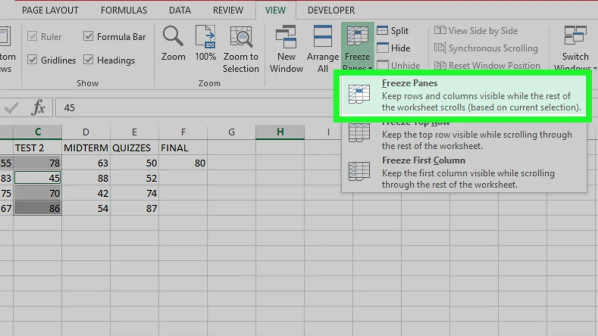
Working on a large spreadsheet in Microsoft Excel on your Mac, you scroll down or across only to lose sight of crucial headers or labels. This can make it harder to understand the data and increase the chance of errors.

This article explains how to freeze panes in Excel on Mac, helping you keep specific rows or columns visible as you navigate your worksheet. You'll learn not just the basic steps but also how the Mac version differs from Windows, including how to handle common Mac-specific challenges.

Key takeaways

Freeze panes by selecting the cell below and to the right of the area you want to keep visible, then choosing Window > Freeze Panes.
Freezing rows or columns separately uses the same Freeze Panes option but requires selecting the correct cell first.
Manual freezing lets you customize exactly which rows and columns stay visible, unlike the fixed options on Windows.
Unfreezing panes is done from the same menu: Window > Unfreeze Panes.
If freezing doesn’t work, check that you’re not in editing mode and that the worksheet is active, as these are common Mac-specific issues.

Before you start: What you need to freeze panes in Excel on Mac

To successfully freeze panes in Microsoft Excel on your Mac, make sure you have a compatible version installed. Freeze Panes is supported on Excel for Mac versions 2016, 2019, and Microsoft 365. Keeping Excel updated ensures you have the latest features and fixes, so check for updates via the Help menu or Microsoft AutoUpdate.

Before freezing panes, take a moment to plan which rows or columns you want to keep visible as you scroll. Understanding your worksheet layout helps you choose the correct cells for freezing. For example, if you want to keep the top header row visible, you will freeze the first row; if you want to keep the first column visible, you freeze that column, or you can freeze both by selecting the appropriate cell.

On Mac, the Freeze Panes options are found under the View tab in the Excel ribbon, which differs slightly from Windows. Instead of the Windows ribbon's View tab, Mac Excel uses a streamlined ribbon, and the Freeze Panes button is located on the right side of the View tab. Familiarize yourself with this location so you can easily access the freezing options.

The Freeze Panes button on Mac offers three options: Freeze Panes, Freeze Top Row, and Freeze First Column. The user interface on Mac may not have as many submenus as Windows, so the options are more direct but require understanding which option fits your needs.

How to freeze panes in Microsoft Excel on Mac

Freezing panes in Excel on a Mac helps you keep specific rows or columns visible as you scroll through your worksheet. To start, open your worksheet and click the cell located just below the rows and just to the right of the columns you want to freeze. For example, if you want to freeze the top row and the first column, select cell B2.

Select the cell below and to the right of the area you want to freeze. After selecting, you should see the cell highlighted, indicating your choice.
Go to the View tab on the Ribbon at the top of the Excel window. This tab contains the options related to window layout and visibility.
Click on the Freeze Panes button. A dropdown menu will appear with several options.
From the dropdown, choose Freeze Panes. This action locks all rows above and columns to the left of your selected cell. You will notice a thin line appearing to indicate the frozen panes.

On Mac Excel, the Freeze Panes command is located in the View tab, unlike Windows Excel, where it is often found under the Window or View tabs depending on the version. Additionally, the Mac version may have slightly different menu wording or layout, so look for the Freeze Panes icon resembling a window split.

For instance, selecting cell B2 and applying Freeze Panes will keep row 1 and column A visible as you scroll down or across. Before freezing, scrolling will move the entire sheet; after freezing, these pane boundaries stay fixed, allowing you to reference headers or key data easily.

Using this method provides a straightforward way to lock rows and columns in place and helps maintain context in large spreadsheets on your Mac.

How to freeze rows in Excel on Mac

Freezing rows in Excel on Mac allows you to keep important information, such as header rows, visible while you scroll vertically through your worksheet. To freeze a single top row, Excel provides a quick option, but if you need to freeze multiple rows, you will use a slightly different approach.

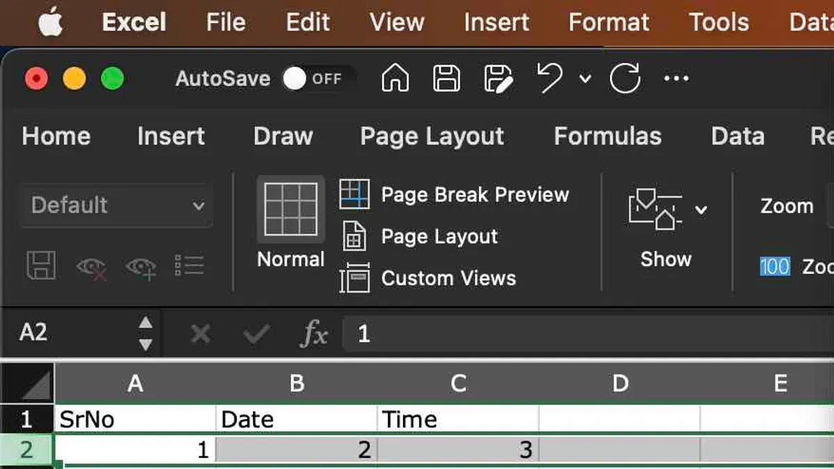
Select the row immediately below the last row you want to freeze. For example, if you want to freeze the first two rows, click on row 3. When you've selected the correct row, it should be highlighted.
Go to the View tab on the Excel ribbon and click on the Freeze Panes dropdown menu. If you want to freeze just the top row, select Freeze Top Row. This will lock the first row only, and as you scroll down, that row remains visible.
If you want to freeze multiple rows, instead of choosing Freeze Top Row, select Freeze Panes from the same dropdown. This freezes all rows above the selected cell, keeping them visible as you scroll.
Scroll down your worksheet to verify that the rows you froze remain visible while the rest of the sheet scrolls. This is particularly helpful when your header information spans several rows, such as a title row followed by column headers.

For example, if your worksheet has a title in row 1 and column headings in row 2, freezing both rows ensures you always see them, which helps keep your data context clear. Freezing only the top row might hide part of your header information if it occupies more than one row.

By selecting the row below the last header row and using the Freeze Panes option, you control exactly which rows stay fixed. This flexibility is useful when working with complex tables or reports where multiple header rows provide essential context.

How to freeze columns in Excel on Mac

Freezing columns in Excel on Mac allows you to keep important columns, like IDs or names, visible while you scroll horizontally through large datasets. This is especially useful when working with wide spreadsheets where you need constant reference to key information. You can freeze a single column or multiple columns depending on your needs.

Select the column immediately to the right of the last column you want to freeze. For example, if you want to freeze columns A and B, select column C. When done correctly, your active cell will be somewhere in that selected column.
Go to the View tab in the Excel ribbon at the top of your screen.
Click on Freeze Panes to open the dropdown menu.
Choose Freeze Panes from the menu. This action locks all columns to the left of the selected column, keeping them visible as you scroll horizontally.

For example, freezing the first column (column A) keeps the ID or name column visible while you move across the sheet. Without freezing, these key reference columns scroll out of view, making it harder to track data. With freezing applied, the frozen columns stay fixed on the left side, and the rest of the worksheet scrolls normally.

The difference between freezing one column and multiple columns is just where you position your cursor before applying Freeze Panes. Selecting the column immediately to the right of the last column you want frozen ensures you lock exactly those columns. If you select only column B, only column A freezes; selecting column D will freeze columns A, B, and C.

Visually, you’ll notice a thin vertical line appear to the right of the frozen columns, indicating where the freeze begins. As you scroll horizontally, frozen columns remain visible on the left side while columns to the right move normally.

How to manually freeze panes in Excel on Mac

When you want to freeze both rows and columns simultaneously or control exactly which parts of your spreadsheet stay visible, you use the manual freeze panes option. This method lets you select an active cell that defines the boundary between frozen and scrolling areas, giving you more flexibility for complex layouts. The key is understanding that the rows above and the columns to the left of the selected cell will be frozen.

For example, if you select cell D5, Excel will freeze rows 1 through 4 and columns A through C. This way, as you scroll down or right, these rows and columns remain visible. This manual approach works well when you need to keep multiple header rows and key columns in view at the same time.

Select the cell below the last row and to the right of the last column you want to freeze. For instance, click on cell D5 to freeze the top 4 rows and first 3 columns.
Go to the View tab on the Excel ribbon.
Click on Freeze Panes in the Window group.
From the dropdown menu, choose Freeze Panes. You should now see a bold line separating the frozen rows and columns from the rest of the sheet.
Test by scrolling down and right; the selected rows above and columns left of your active cell stay visible.

This manual freeze pane option is especially useful when your worksheet includes multiple header rows and columns that must remain visible simultaneously. Keep in mind that the selected cell sets the freeze boundary, so selecting the wrong cell might freeze too few or too many rows or columns.

How to unfreeze panes in Excel on Mac

Unfreezing panes in Excel on Mac is a straightforward way to restore normal scrolling behavior when you no longer need specific rows or columns to stay visible. This process is helpful when you want to adjust which parts of your worksheet are frozen or if you encounter display issues caused by frozen panes. Removing the freeze settings allows you to start fresh with new freeze selections.

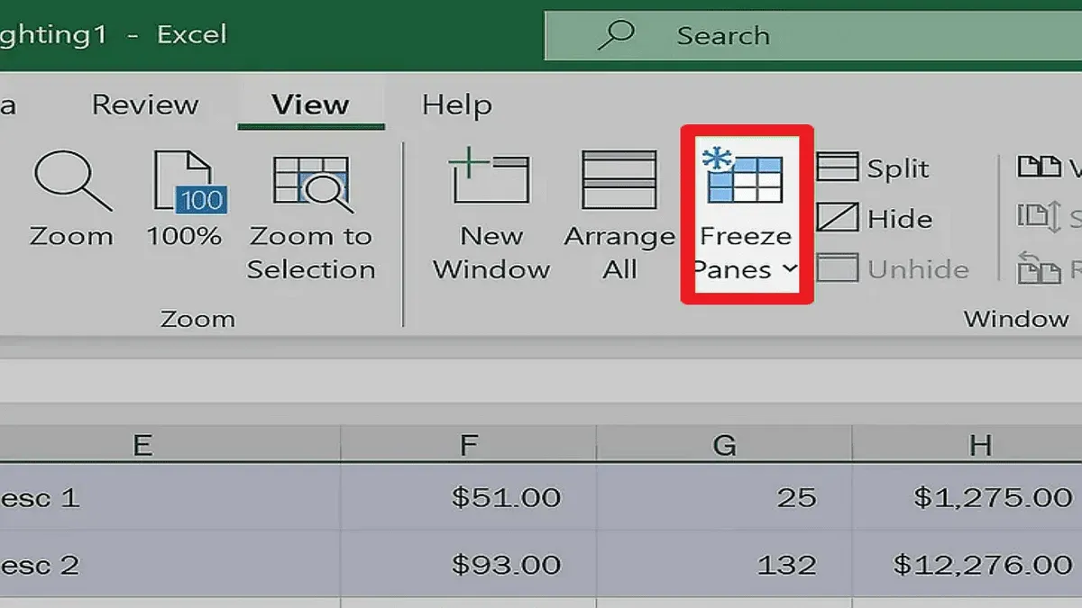
Click on the View tab in the Excel ribbon at the top of your screen. This reveals options related to worksheet display.
Locate and click the Freeze Panes button within the View tab. A drop-down menu will appear.
Select Unfreeze Panes from the drop-down menu. When successful, any frozen rows or columns will become unfrozen, allowing all worksheet cells to scroll freely.

After unfreezing, you can confirm the change by scrolling vertically and horizontally to see that no rows or columns remain locked in place. For example, if you initially froze the top row and left column but now want to freeze just the first two rows, you must unfreeze first, then select the appropriate cell and freeze panes again.

Before unfreezing, your worksheet might show a thick grey line indicating the frozen areas. After unfreezing, this line disappears, and the worksheet scrolls normally without locked rows or columns.

If you experience unexpected freezing behavior or your panes don’t freeze correctly, unfreezing and then resetting the freeze selection often resolves the problem.

Troubleshooting: Why Excel panes are not freezing or freezing incorrectly on Mac

If Excel panes are not freezing as expected on your Mac, the issue often starts with cell selection. Freezing panes relies on selecting the correct cell or row/column boundary before activating Freeze Panes. Selecting a cell too far right or too far down can cause unexpected freezing behavior, such as freezing more panes than intended or freezing the wrong rows or columns.

Worksheet protection settings can also interfere. If your worksheet or workbook is protected, Excel may prevent changes to pane freezing. You might see an error message like "This command is not available because the worksheet is protected." To fix this, unprotect the sheet via the Review tab before trying to freeze panes again.

Another cause of freeze panes malfunction is outdated Excel software or bugs specific to Mac versions. If freezing panes fails silently or behaves erratically, check for updates through Help > Check for Updates. Applying the latest updates can resolve many glitches related to pane freezing.

Macros that manipulate freeze panes in Excel for Windows may not always work correctly on Mac due to differences in VBA support and interface. If you rely on macros, verify compatibility and test the freeze panes commands manually to confirm they operate as intended on Mac.

When freeze panes options become unresponsive, restarting Excel or rebooting your Mac can clear temporary software glitches affecting the feature. This simple step often restores normal freezing functionality if no other settings are blocking it.

Select the cell just below and to the right of where you want the freeze to occur, then activate Freeze Panes from the View tab. You should see the pane lines appear correctly.
If freezing fails, check if the worksheet is protected by going to the Review tab and selecting Unprotect Sheet. Try freezing panes again.
Verify your Excel version via Help > About Excel and update if necessary using Help > Check for Updates.
Test freezing panes manually to rule out macro issues if you use VBA scripts to control freezing.
Close Excel and reopen it; if the problem persists, restart your Mac to clear any stalled processes.

Following these steps helps identify and fix common reasons why freezing panes might not work or behave unexpectedly on Mac Excel.

Frequently asked questions

How to freeze panes in ms excel?

To freeze panes in MS Excel, select the cell below and to the right of the rows and columns you want to keep visible. Then go to the View tab on the ribbon and click on Freeze Panes. Choose the appropriate option based on whether you want to freeze the top row, first column, or a custom pane.

How to freeze panes in excel pc?

On a PC, open your Excel workbook and select the cell where you want the freeze to begin. Navigate to the View tab, click Freeze Panes, and then select Freeze Panes from the dropdown menu. This locks all rows above and columns to the left of your selected cell.

How to do freeze panes in excel?

Freezing panes in Excel involves selecting a specific cell, then using the Freeze Panes option under the View tab. This action keeps rows above and columns to the left of that cell visible while scrolling through your worksheet.

How to freeze panes in excel on macbook?

On a MacBook, open Excel and select the cell below and to the right of the area you want to freeze. Then, go to the Window menu in the top toolbar, choose Freeze Panes, and select Freeze Panes again. This process differs slightly from Windows but achieves the same result.

How to freeze panes in MS Excel on MacBook?

In MS Excel on a MacBook, click the cell where you want to begin freezing panes. Then, from the top menu, select Window > Freeze Panes > Freeze Panes. This will lock the rows above and columns to the left of the selected cell, keeping them visible as you scroll.

What This Guide Does Not Cover

This guide covers standard Excel freeze panes functionality on Mac and does not address advanced VBA macros beyond basic freeze pane automation, nor does it cover Excel alternatives or older Excel versions that lack freeze panes support. If you require complex automation or are using significantly outdated software, specialized resources or updated versions of Excel might be necessary. Additionally, this article focuses on native Excel behavior on Mac and does not explore third-party add-ins or tools.

To master freeze panes on your Mac effectively, the best next step is to practice freezing different rows and columns in your own spreadsheets. Try selecting various cells before applying freeze panes and observe how Excel locks the rows or columns relative to your selection. This hands-on approach will deepen your understanding and help you tailor the feature precisely to your workflow needs.