Spreadsheets

How to Freeze Header Rows in Numbers: A Step-by-Step Guide

Discover step-by-step how to freeze header rows in Numbers on Mac and iPad to keep your headers visible while working with large spreadsheets.

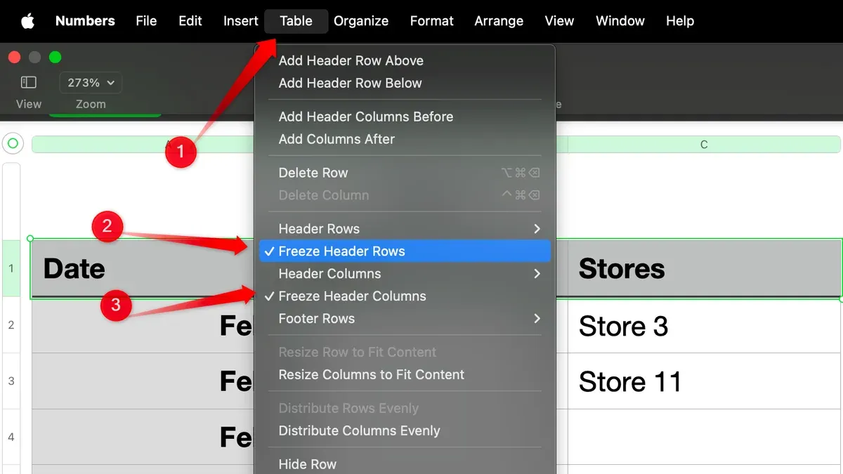
Working with large spreadsheets in Numbers can be frustrating when your column headers disappear as you scroll down. You might wonder how to keep those header rows visible, especially if you’re used to Excel’s way of freezing panes. This article explains how to freeze header rows in Numbers, both on Mac and iPad, so you can always see your labels while navigating your data.

You’ll learn step-by-step methods tailored to each device, understand what freezing headers means in Numbers, and get tips when the feature doesn’t work as expected. Additionally, this guide compares Numbers’ approach with Excel’s, helping you decide the best way to manage frozen rows for your workflow.

Key takeaways

Use the Table menu’s “Freeze Header Rows” option on Mac to lock header rows in place.
On iPad, tap the table, then use the Format sidebar to freeze header rows.
Freezing headers keeps the top row visible during vertical scrolling but does not lock columns.
If freezing doesn’t work, check that your table has header rows defined and isn’t grouped.
Numbers freezes headers differently from Excel, focusing on table-specific settings rather than window panes.

Before you start: What you need to freeze header rows in Numbers

To freeze header rows in Apple Numbers, first ensure you have the app installed on a compatible device. Numbers is available on Mac computers running macOS Mojave (10.14) or later, and on iPads with iPadOS 13 or later. The freezing feature works smoothly on these platforms, but earlier versions may not support it fully or at all.

Understand that Numbers handles header rows differently than Excel. Instead of "freezing panes" like in Excel, Numbers uses a table structure where header rows are locked to keep them visible. This means you’ll be "locking" the header rows within a table rather than freezing sections of the sheet.

While the underlying concept of keeping header rows visible remains the same, the steps to achieve this differ between Mac and iPad. Knowing this helps you follow instructions precisely based on your device.

Before proceeding, have a spreadsheet open in Numbers with at least one table that includes the header rows you want to keep visible. This setup is essential to practice the freezing steps directly.

Open Apple Numbers on your Mac or iPad. You should see the main interface with your documents or the option to create a new one.
Open an existing spreadsheet or create a new one, ensuring it contains a table with header rows. Header rows usually label columns and are at the top of each table.
Confirm that your Numbers app version supports freezing headers by checking for header row options in the table formatting sidebar or toolbar. If these options are unavailable, update your app to the latest version.

How to freeze header row in Numbers on Mac

Freezing header rows in Numbers on your Mac helps keep important column titles visible as you scroll through large tables. This makes it easier to understand your data at a glance. Follow these steps to freeze header rows effectively.

Select the table by clicking anywhere inside it. When selected, the table border will highlight, indicating it is active.
Open the Table sidebar by clicking the paintbrush icon in the top right corner of the Numbers window. This reveals formatting options specific to tables.
Locate the Header Rows setting under the Table tab in the sidebar. You will see a field labeled “Header Rows” with a number input.
Set the number of header rows to freeze by entering the number of top rows you want to lock in place, typically “1” for a single header row. When you do this, those rows become designated as headers and stay visible when you scroll vertically.
Verify the freeze by scrolling down your table. The header row(s) you specified remain fixed at the top while the rest of the rows scroll underneath.

If you want to freeze multiple header rows, simply increase the number in the Header Rows field. For example, entering “2” will lock the top two rows as headers. This is useful if your table has a multi-row header with grouped categories.

Note that frozen header rows are visually indicated by a slight shading difference and a thin line beneath them. This helps you distinguish header rows from the rest of the data. If you do not see the header rows stay put when scrolling, double-check your table is selected and the Header Rows number is set correctly.

Unlike Excel’s pane freezing, Numbers handles header rows as a table property rather than a window feature. This means header rows remain frozen only within each table, not across multiple tables or the entire sheet.

How to freeze header row in Numbers on iPad

Freezing header rows in Numbers on your iPad helps keep important labels visible as you scroll through your spreadsheet. The iPad interface differs from Mac, so here’s how to do it step by step.

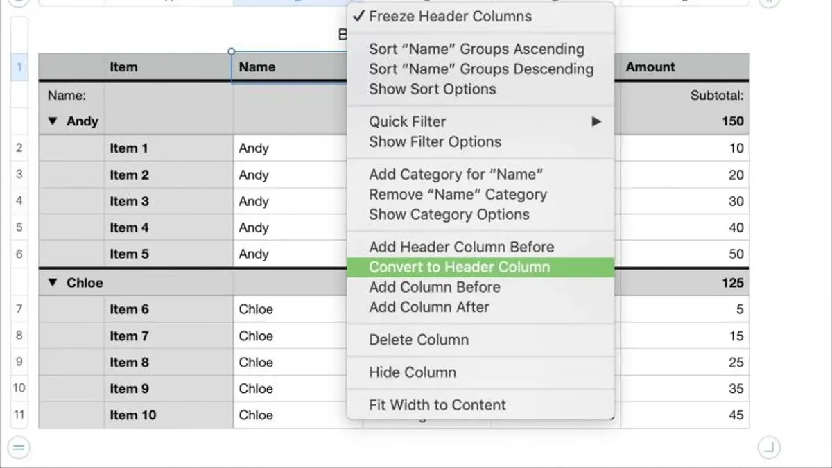
Open your spreadsheet in Numbers and tap once on the table containing the header rows you want to freeze. You should see the table highlighted with selection handles around it.
Tap the Format button, which looks like a paintbrush icon, located in the upper right corner of the screen. This opens the Format panel specific to the selected table.
In the Format panel, scroll down or look for the Table section. Here, find the Header Rows option. It will show a number representing how many top rows are currently frozen or available to freeze.
Tap the Header Rows option and increase the number by tapping the plus icon or entering a number to freeze the desired number of top rows. Typically, Numbers on iPad lets you freeze one or more header rows, but the maximum may vary depending on the table structure.
After setting the header rows, scroll vertically within your table. You should see the frozen header rows stay visible at the top while the rest of the rows move underneath them.

Compared to Mac, the iPad uses the Format panel instead of a sidebar, and you interact through touch rather than clicking menus. While the Mac allows quick adjustments via the sidebar, the iPad’s method is slightly more hidden but straightforward once you find the Header Rows setting. Keep in mind the number of header rows you can freeze at once on iPad may be limited to a few rows, unlike Excel’s more flexible freeze pane features.

What does freeze header rows mean in Numbers

Freezing header rows in Numbers means locking the top rows of a table so they remain visible as you scroll through the rest of your data. This feature helps you easily keep track of column labels or key information without losing context when working with large spreadsheets. Unlike Excel’s freeze panes, which lock specific rows or columns across the entire worksheet, Numbers treats header rows as a property of the individual table.

When you freeze header rows in Numbers, only those rows within the selected table stay fixed. Scrolling beyond the table or switching to another table does not preserve those headers. This design ensures that each table can have its own header configuration, but it also means freezing isn’t applied worksheet-wide.

For example, imagine a table with 50 rows of data. Without frozen header rows, when you scroll down, the column titles disappear, making it harder to interpret the data. When you set 1 or more header rows to freeze, those rows remain visible at the top of the table while you scroll through the remaining rows. This clarity speeds up data entry and analysis by keeping important context in view.

In contrast, Excel’s freeze panes lock rows and columns based on your selection, affecting the whole worksheet view regardless of table boundaries. Numbers’ approach focuses on table-level control, which can be simpler but requires you to set header rows individually for each table you want fixed headers in.

How to freeze rows in Numbers beyond headers

In Numbers, freezing is limited to locking the top rows as headers. You cannot freeze arbitrary rows in the middle of a table the way Excel allows with its freeze panes feature. This means if you want to keep specific rows visible beyond the designated header rows, you need to use workarounds.

One common approach is to split your data into multiple tables. For example, you can place important rows you want always visible in a separate table above your main data table. This keeps those rows accessible while scrolling through the larger dataset below. It requires some manual organization but effectively mimics freezing key rows beyond headers.

Another option is using filters to temporarily focus on relevant parts of your data. While filters do not freeze rows, they reduce visible content, helping you keep important rows in view. However, this changes what data you see rather than locking rows in place.

Feature	Numbers	Excel
Freeze top header rows	Yes	Yes
Freeze arbitrary rows mid-table	No	Yes
Split data into multiple tables as workaround	Yes	Rarely needed

To organize data effectively in Numbers, consider placing frequently referenced rows in dedicated tables or sections. Label these tables clearly to maintain context. This method helps you keep essential information visible without relying on unsupported freeze options.

Select the rows you want to keep visible beyond the header rows and copy them.
Create a new table above or beside your main table by clicking the + button and choosing Table.
Paste the copied rows into this new table.
Adjust the size and position of both tables so you can scroll through the main data while the separate table remains visible.
Label the new table clearly to indicate its contents, helping you track important information at a glance.

How to freeze header rows in Numbers when it’s not working

If freezing header rows in Numbers isn’t working as expected, start by confirming that you’ve selected the correct table. Header row freezing only affects tables, so clicking outside the table or selecting charts or other objects won’t enable this feature. Next, check the sidebar on Mac or the Format panel on iPad to ensure that header rows are actually enabled and that you’ve set a number greater than zero for header rows.

Another common issue is using a view mode that disables header freezing. For example, some filtered or grouped views can interfere with freezing behavior. Switch back to a standard view to test whether header rows freeze properly. Also, verify that the rows you want frozen are defined as header rows, not simply styled to look like headers. Only designated header rows are locked when scrolling.

If these steps don’t resolve the issue, restart Numbers to clear temporary glitches. Check for updates and install the latest version of the app, as freezing features might not work correctly on outdated software. Remember that freezing header rows applies strictly within tables; it does not work on charts, images, or other inserted objects within your spreadsheet.

Select the table where you want to freeze header rows. When done correctly, the table’s blue outline will appear around it.
Open the Table sidebar on Mac or the Format panel on iPad, locate the Header Rows setting, and set it to at least 1. The header rows should highlight to confirm selection.
Ensure you are not in a filtered or grouped view by switching to the default table view. The frozen headers should now stay visible when you scroll.
If freezing still does not work, close and reopen Numbers, then try again. This often resolves unresponsiveness.
Check for app updates in the App Store and install any available updates; freezing features improve with newer releases.

By following these steps, you can identify and fix the typical reasons why header row freezing might fail or behave unexpectedly in Numbers.

How freezing header rows in Numbers compares to Excel

When transitioning from Excel to Numbers, understanding how each app handles freezing rows and columns helps you choose the right tool for your workflow. Excel offers a versatile Freeze Panes feature, allowing you to lock any combination of rows and columns at arbitrary positions across the worksheet. In contrast, Numbers limits freezing to the top header rows within individual tables and does not support freezing columns or arbitrary rows beyond these headers.

Feature	Excel	Numbers
Freeze location	Anywhere in the worksheet (rows and columns)	Only top header rows within each table
Freeze columns	Yes	No
Freeze arbitrary rows	Yes	No, only header rows
Integration with table design	Worksheet-wide, independent of table structure	Built into the table settings, affecting only that table

Excel’s flexibility suits complex spreadsheets where you need to keep multiple sections visible simultaneously, such as freezing both header rows and key columns to track data easily. Numbers’ approach works well for simpler tables or when you want a clean interface focused on one table at a time. For example, if you primarily work with single tables and want to keep top headers visible while scrolling vertically, Numbers’ header row freezing is sufficient.

However, if your workflow involves large worksheets with multiple tables, or you require locking columns alongside rows, Excel’s Freeze Panes offers a more adaptable solution. Numbers emphasizes simplicity and table-based design, so freezing is tightly coupled with the header rows concept rather than arbitrary freeze points.

In summary, choose Numbers when your data is organized in distinct tables and you only need to lock top headers. Opt for Excel when your data layout requires freezing multiple rows and columns anywhere on the sheet for enhanced navigation.

Frequently asked questions

How to freeze header rows in excel?

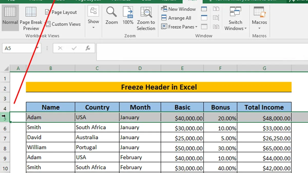
In Excel, you freeze header rows by selecting the row immediately below the headers you want to freeze. Then go to the View tab and click on Freeze Panes. Choose 'Freeze Top Row' to keep the very first row visible or select 'Freeze Panes' to lock multiple rows above your selection. This keeps your headers visible as you scroll through your worksheet.

How to freeze headers in excel?

To freeze headers in Excel, use the Freeze Panes feature under the View tab. If your headers are in the first row, simply click 'Freeze Top Row.' If your headers span multiple rows, select the row below them, then click 'Freeze Panes' to lock all rows above your selection. This way, the headers stay in place while you scroll down.

How to freeze header rows in apple numbers?

In Apple Numbers, header rows are frozen automatically when you designate rows as header rows. To do this, select the rows you want as headers, then open the Table menu and choose 'Header Rows' to set the number of header rows. These header rows stay visible when you scroll vertically. Numbers does not use a separate freeze pane feature like Excel.

How to freeze header in numbers?

Freezing headers in Numbers involves setting header rows in your table. Select the rows at the top of your table you want to keep as headers, then from the Table menu, adjust the 'Header Rows' count. Once set, these rows remain visible as you scroll down the sheet, providing consistent context for your data.

How to freeze excel header row?

To freeze the header row in Excel, click on the View tab, then select 'Freeze Panes' and choose 'Freeze Top Row.' This will lock the first row of your worksheet so it remains visible when scrolling. This is helpful for keeping column labels in view during data analysis.

What This Guide Does Not Cover

This article does not cover freezing columns or arbitrary rows beyond header rows in Numbers, as the app currently does not support those features. If you need to freeze columns or multiple non-header rows, you may find those options available in other spreadsheet applications like Microsoft Excel. Additionally, this guide does not address advanced scripting or automation for freezing rows, which requires different tools or workflows.

For users who require more complex freezing capabilities or who frequently switch between different spreadsheet software, exploring Excel’s freeze panes feature might be the best next step. Numbers focuses on simplicity and usability but has limitations in this area compared to Excel.

To continue improving your spreadsheet navigation in Numbers, the single most useful next step is to practice using header rows effectively by setting up your tables with clearly defined headers and experimenting with freezing them on both Mac and iPad. Becoming familiar with these steps will make your data easier to analyze and navigate.